Double Descent

Part 1: A Visual Introduction

Jared Wilber & Brent Werness, December 2021

Note - this is part 1 of a two article series on Double Descent. Part 2 is available here.

In our previous discussion of the bias-variance tradeoff, we ended with a note about one of modern machine learning’s more surprising phenomena: double descent. Double descent is interesting because it appears to stand counter to our classical understanding of the bias-variance tradeoff. Namely, while we expect the best model performance to be obtained via some balance between bias (underfitting) and variance (overfitting), we instead observe strong test performance from very overfit, complex models. As a result, many practitioners and researchers are left questioning the relevance of the traditional bias-variance tradeoff in modern machine learning.

Here, we'll first introduce the phenomenon for a general example and then offer a soft explanation for why it's occurring. (In a follow up article, we'll describe the phenomena in more low level, mathematical detail).

At the end of it all, we conclude that the double descent phenomenon actually reinforces the importance of the bias-variance tradeoff.

Plotting the training and testing error against some measure of model complexity (say, training time) for a typical case may look like in this figure, with both following the same decreasing direction and the test error hovering slightly above the train error.

Under the classical bias-variance tradeoff, as we move further right along the x axis (i.e. increasing the complexity of our model), we overfit and expect the test error to skyrocket further and further upwards even as the train error continues decreasing.

However, what we observe is quite different. Indeed the error does shoot up, but it does so before descending back down to a new minimum. In other words, even though our model is extremely overfitted, it has achieved its best performance, and it has done so during this second descent (hence the name, double descent)!

We call the under-parameterized region to the left of the second descent the classical regime, and the point of peak error the interpolation threshold. In the classical regime, the bias-variance tradeoff behaves as expected, with the test error drawing out the familiar U-shape.

To the right of the interpolation threshold, the behavior changes. We call this over-parameterized region the interpolation regime. In this regime, the model perfectly memorizes, or interpolates, the training data. That is, every model passes exactly through the given training data, thus the only thing that changes is how the model connects the dots between these data points.
What's Going On?

To better understand this phenomenon, let's explore it together! Quick note - in this article, we'll keep things fairly high-level. However, if you're interested in more mathematical, lower-level details, check out our sibling article on double descent.

Let's begin with a simple problem. We will train on data sampled from a cubic curve that has been occasionally corrupted with noise. We will generate a tiny training set and a larger test set so that we can rapidly explore what is going on, while still trusting the values for the test error, which is obtained from predictions on the test set. To maximize the stability of training, we will not employ a full neural network, but rather pick random non-linear features and then train a linear model on top.

Below we show our data, as well as each model's associated mean absolute error (MAE).


To begin, we plot a simple model. Recall from our previous discussion on the bias-variance tradeoff that basic models cannot capture complex patterns in the data and are thus underfitted, providing poor performance for the task at hand.

Next, we plot a model that's not too simple, nor too complex. It is in this complexity region where, traditionally, we expect to find the best performing model. This is reflected in the low error ( ≤ 0.25) in the bottom chart.

Now, let's plot a complex model, one where our number of features is equal to the number of dimensions. This situation, in which the model passes through each and every point in the training set, is our interpolation threshold. At this stage we're overfitting, which leads to the high test error shown in the plot. Typically, we would stop increasing the complexity here and revert to a more simple model that achieves a good tradeoff between bias and variance.

The existence of the double descent phenomenon means that this picture is incomplete. We stopped making more and more intricate models when we reached a certain complexity level. But what happens if we go further, beyond the interpolation threshold? Let's look at a single example with 256 random features and what happens with the test error curve as we extend to that situation.

The test MAE is even lower for these large models! The traditional U-shape is sometimes telling only part of the story. Past the traditional U-shaped region is the interpolation regime. The idea is that every model past that spike in error is complex enough to pass through every single training data point, thus all models are interpolating the training set. More complicated models can achieve smoother interpolations. If the conditions are right (as they are in this experiment) these enormous interpolating models can perform far better than traditional well-fit models.

Try for yourself! Toggle the slider to modify the number of non-linear features used to build the models.


Minding The Gap

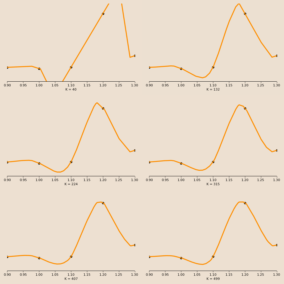
Image of interpolation region from above.

It's important to pay attention to the gap between the points once we've entered our interpolation region (K > 36). In the image to the left, we show, for a small portion of the data above, how the interpolation varies across 40 to 500 features.


Once we're at the interpolation threshold, every model from that complexity level onwards passes through each training data point. The only thing that changes is how the model connects the in-between points. As the models become more and more complex, these connections can become smoother, and the resulting prediction may fit your test data better. This is why models in the interpolation region can perform so well.

Final Takeaways


The key takeaway here is that double descent is a real phenomenon, although its existence does not nullify the bias-variance tradeoff. It is believed that double descent contributes to explain why deep neural networks perform so well at many tasks. By building models with many more parameters than data points, deep neural networks are often operating in this interpolating regime. Traditional intuition from the bias-variance tradeoff would discourage such approach, indicating that simpler models with fewer parameters should be more performant. However, this has been contradicted with experiments. Double descent provides an indication that even though models that pass through every training data point are indeed overfitted, the structure of the resulting network forces the interpolation to be smooth and results in superior generalization to unseen data.


Thanks for reading! If you've made it this far, consider viewing our follow-up article explaining double descent in more detail. To learn more about machine learning, check out our self-paced courses, our youtube videos, and the Dive into Deep Learning textbook. If you have any comments or ideas related to MLU-Explain articles, feel free to reach out directly. The code for this article is available here.

References & Open Source

This article is a product of the following resources + the awesome people who made (& contributed to) them: